담금질 기법
어떤 문제를 풀고자 할 때, 풀고자 하는 공간의 정보가 부족하거나 연속적이지 않으면, 뉴턴 방법과 같은 방법은 사용할 수 없습니다(야코비안 같은 미분 행렬 계산이 필요합니다.). 이런 경우에 확률적 탐색 기법를 시도해 볼 수 있습니다. 특히 이 방법들은, 조합적 최적화 문제를 푸는 데 빈번히 사용됩니다. 이러한 문제의 예로 외판원 문제가 있습니다.
문제 공간에서 해를 구한다는 것은 실수 값을 가지는 에너지 함수 (비용 함수라고도 합니다)의 값이 최소화되는 지점을 찾는 것을 의미합니다. 담금질 기법(Simlated annealing)은 지역적 최소화를 피할 수 있어 일반적으로 좋은 결과를 내놓는 최소화 기법입니다. 이 방법은 온도(temperature)를 낮출 수 있는 무작위 전이를 공간 위에서 진행합니다. 각 걸음의 진행 확률은 볼츠만 분포에 의해 결정됩니다.
이 단원에서 기술된 함수들은 gsl_siman.h 헤더파일에 기록되어 있습니다.
담금질 알고리즘
담금질 알고리즘은 기본적으로 문제 공간에서 무작위 방향 중 에너지를 최소화하는 경향으로 상태를 확률적으로 바꾸며 해를 탐색합니다. 이러한 전이 확률은 볼츠만 분포을 기반으로 결정됩니다.
\(E_{i+1} >E_i\) 인 조건에서 성립하며, \(E_{i+1} \leq E_i\) 인 경우 \(p=1\) 로 정의합니다.
다시 말해, 새로운 에너지 단계가 낮으면 전이가 일어나고, 새로운 에너지 단계가 높으면 확률에 기반해 전이가 결정됩니다. 이 확률은 온도 \(T\) 에 비례하고, 에너지 차이 \(E_{i+1}-E_i\) 에 반비례합니다.
온도 \(T\) 는 초기 단계에서 결정되며 일반적으로 적절한 높은 값을 가집니다. 무작위 전이는 이 온도 값에 의존하게 됩니다. 전이 과정에서 온도는 설계된 냉각 절차에 따라 천천히 낮아집니다. 예를 들어 \(T -> T/ \mu_T\) 으로 \(\mu_T\) 를 1보다 조금 더 큰 수로 설정해 볼 수 있습니다.
이러한 높은 에너지 상태로 전이할 수 있는 확률의 존재는 다양한 상황에서 담금질 기법이 지역적 최소값에 빠지지 않도록 해, 최적의 값을 찾을 수 있도록 도와줍니다.
담금질 함수
-
void gsl_siman_solve(const gsl_rng *r, void *x0_p, gsl_siman_Efunc_t Ef, gsl_siman_step_t take_step, gsl_siman_metric_t distance, gsl_siman_print_t print_position, gsl_siman_copy_t copyfunc, gsl_siman_copy_construct_t copy_constructor, gsl_siman_destroy_t destructor, size_t element_size, gsl_siman_params_t params)
주어진 공간에서 담금질 기법을 이용해 해를 찾습니다. 공간은
Ef와distance로 정의됩니다. 각 전이 단계는 주어진 인자 중 난수 생성자r과 함수take_step에 의해 결정됩니다.이 계의 시작 조건 설정은
x0_p에 의해 주어집니다. 이 명령어 집합은 2개의 방법으로 현재 설정을 갱신하는데, 고정 크기 방법 (fixed-size mode)과 동적 크기 방법 (variable-size mode)이 있습니다. 고정 크기 방법에서는 설정이 메모리 상의element_size크기의 한 공간에 저장되고, C의 표준 함수malloc(), memcpy(), free()들에 의해 내부에서 이 설정의 복사본들의 생성, 복사, 소멸이 진행됩니다. 이 고정 크기 방법 상태에서는 함수 포인터copyfunc, copy_constructor그리고destructor이null값을 가지게 됩니다. 반면, 동적 크기 방법에서는copyfunc, copy_constructor그리고destructor들이malloc(), memcpy(), free()대신에 쓰입니다. 이 경우element_size값은 0으로 주어집니다.params구조체 변수(세부 구조는 후술)는 제공된 온도 계획과 수정 가능한 변수들로 이루어지는 실행을 제어합니다.종료 시, 알고리즘 과정을 통해 얻어진 최적의 결과가
x0_p에 저장됩니다. 만약, 담금질 기법이 성공적이었다면, 이는 문제 공간의 최적점에 대해 좋은 근사를 나타내줍니다.만약, 함수 포인터
print_position가NULL값이 아니라면, 디버그 기록이stdout에 출력될 것입니다. 이는 다음과 같은 행을 가집니다:#-iter #-evals temperature position energy best_energy
함수
print_position의 출력 값도 같이 출력됩니다. 만약print_position가NULL이라면, 아무 값도 출력 되지 않습니다.
이 라이브러리의 담금질 알고리즘 명령어 집합은 사용자 정의 함수들을 필요로 합니다. 해당 함수들은 풀고자 하는 문제 공간과 에너지 함수를 정의합니다. 이러한 함수들을 사용자가 직접 다음의 초안의 형태로 정의해 풀고자하는 문제에 적절한 함수들을 스스로 선택해 알고리즘에 사용할 수 있습니다.
-
type gsl_siman_Efunc_t
현재 상태
xp에 대한 에너지를 반환해야 합니다.double (*gsl_siman_Efunc_t) (void *xp)
-
type gsl_siman_step_t
현재 상태
xp를 난수 발생자r와 단계별 최대 이동거리step_size를 이용해 수정해야 합니다.void (*gsl_siman_step_t) (const gsl_rng *r, void *xp, double step_size)
-
type gsl_siman_metric_t
주어진 두 개의 상태
xp와yp사이의 거리를 반환해야 합니다.double (*gsl_siman_metric_t) (void * xp, void * yp)
-
type gsl_siman_print_t
주어진 상태
xp의 설정값을 출력해야 합니다.void (*gsl_siman_print_t) (void *xp)
-
type gsl_siman_copy_t
설정 값을
source에서dest로 복사해야 합니다.void (*gsl_siman_copy_t) (voi d *souirce, coid *dest)
-
type gsl_siman_copy_construct_t
설정
xp의 새 복사본을 만들어야 합니다.void (*gsl_siman_copy_construct_t) (void *xp)
-
type gsl_siman_destroy_t
설정
xp를 삭제해야 합니다. 다시말해,xp가 들어있는 메모리를 해제해야 합니다.void (*gsl_siman_destroy_t) (void *xp)
-
type gsl_siman_params_t
gsl_siman_solve()의 실행을 제어하는 인자들입니다. 이 구조체는 탐색, 에너지 함수, 단계 함수와 초기 가정을 제어하는 데 필요한 모든 정보를 담고 있습니다.int n_tries각 단계에서 시도할 지점의 수.
int iters_fixed_T각 온도별 반복 횟수.
double step_size각 무작위 전이에서 최대 크기.
double k, t_initial, mu_t, t_min볼츠만 분포 인자들과 냉각 절차 인자.
예제
GSL의 담금질 알고리즘 구현은 그다지 세련된 구현체가 아닙니다. 상당히 원시적인 형태로 구현되어 있습니다. 이는 의도된 사항입니다. 이 구현체는 C로 작성해 C에서 호출함을 염두에 두고 개발되었으며, 동시에 다양한 응용 가능성에 목적을 두고 있기 때문입니다. 그렇기에 여기서 라이브러리의 사용자들이 개발하는 응용 프로그램에 약간의 수정을 거쳐 적용할 수 있는 여러 예시들을 제공할 것입니다. 이는 다양한 구현을 좀 더 쉽게 할 수 있도록 도와줄 것입니다.
Trivial 예제
첫번째 예제로, 1차원 직교 좌표계에서 감쇠하는 sine 함수를 에너지 함수로 둔 상황을 살펴봅시다. 이 공간은 많은 지역적 최소값이 존재합니다. 하지만 전역 최소값은 1개만이 존재합니다. 1.0과 1.5사이에 이 값이 존재합니다. 초기 추정은 15.5입니다. 전역 최소값으로 부터 사이에 여러 지역적 최소값이 존재하는 지점입니다.
#include <math.h>
#include <stdlib.h>
#include <string.h>
#include <gsl/gsl_siman.h>

/* set up parameters for this simulated annealing run */

/* how many points do we try before stepping */
#define N_TRIES 200

/* how many iterations for each T? */
#define ITERS_FIXED_T 1000

/* max step size in random walk */
#define STEP_SIZE 1.0

/* Boltzmann constant */
#define K 1.0

/* initial temperature */
#define T_INITIAL 0.008

/* damping factor for temperature */
#define MU_T 1.003
#define T_MIN 2.0e-6

gsl_siman_params_t params
  = {N_TRIES, ITERS_FIXED_T, STEP_SIZE,
     K, T_INITIAL, MU_T, T_MIN};

/* now some functions to test in one dimension */
double E1(void *xp)
{
  double x = * ((double *) xp);

  return exp(-pow((x-1.0),2.0))*sin(8*x);
}

double M1(void *xp, void *yp)
{
  double x = *((double *) xp);
  double y = *((double *) yp);

  return fabs(x - y);
}

void S1(const gsl_rng * r, void *xp, double step_size)
{
  double old_x = *((double *) xp);
  double new_x;

  double u = gsl_rng_uniform(r);
  new_x = u * 2 * step_size - step_size + old_x;

  memcpy(xp, &new_x, sizeof(new_x));
}

void P1(void *xp)
{
  printf ("%12g", *((double *) xp));
}

int
main(void)
{
  const gsl_rng_type * T;
  gsl_rng * r;

  double x_initial = 15.5;

  gsl_rng_env_setup();

  T = gsl_rng_default;
  r = gsl_rng_alloc(T);

  gsl_siman_solve(r, &x_initial, E1, S1, M1, P1,
                  NULL, NULL, NULL,
                  sizeof(double), params);

  gsl_rng_free (r);
  return 0;
}
그림 12 는 siman_test 를 다음과 같이 실행한 결과입니다.
$./siman_test | awk '!/^#/ {print $1, $4}'
 | graph -y 1.34 1.4 -W0 -X generation -Y position
 | plot -Tps > siman-test.eps
그림 13 는 siman_test 다음과 같이 실행한 결과입니다.
$./siman_test | awk '!/^#/ {print $1, $5}'
 | graph -y -0.88 -0.83 -W0 -X generation -Y energy
 | plot -Tps > siman-energy.eps
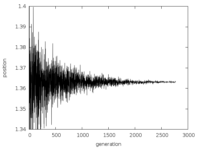
그림 12 담금질 방법 실행 예시: 높은 온도에서(그래프 시작지점)는 해가 여러 값으로 발산하는 것을 볼 수 있습니다. 하지만 낮은 온도에서는 수렴합니다.
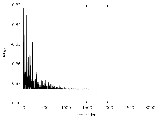
그림 13 담금질 방법 에너지 vs 시행 횟수
외판원 문제
외판원 문제는 고전적인 조합적 최적화 문제입니다. Mark Galassi는 미국 남부 도시 12개의 좌표를 기반으로 아주 간단한 형태의 외판원 문제를 제시했습니다. 이 문제는 엄밀히 말해 비행기를 탄 외판원 문제입니다. 도시와 도시 사이의 거리를 기반으로 하고, 실질적인 차량의 이동거리를 기반으로 하지 않았기 때문입니다. 때문에, 지오이드 거리 1 를 적용하지 않았습니다.
전체 코드는 다음과 같습니다.
/* siman/siman_tsp.c
 *
 * Copyright (C) 1996, 1997, 1998, 1999, 2000 Mark Galassi
 *
 * This program is free software; you can redistribute it and/or modify
 * it under the terms of the GNU General Public License as published by
 * the Free Software Foundation; either version 3 of the License, or (at
 * your option) any later version.
 *
 * This program is distributed in the hope that it will be useful, but
 * WITHOUT ANY WARRANTY; without even the implied warranty of
 * MERCHANTABILITY or FITNESS FOR A PARTICULAR PURPOSE.  See the GNU
 * General Public License for more details.
 *
 * You should have received a copy of the GNU General Public License
 * along with this program; if not, write to the Free Software
 * Foundation, Inc., 51 Franklin Street, Fifth Floor, Boston, MA 02110-1301, USA.
 */

#include <config.h>
#include <math.h>
#include <string.h>
#include <stdio.h>
#include <gsl/gsl_math.h>
#include <gsl/gsl_rng.h>
#include <gsl/gsl_siman.h>
#include <gsl/gsl_ieee_utils.h>

/* set up parameters for this simulated annealing run */

#define N_TRIES 200             /* how many points do we try before stepping */
#define ITERS_FIXED_T 2000      /* how many iterations for each T? */
#define STEP_SIZE 1.0           /* max step size in random walk */
#define K 1.0                   /* Boltzmann constant */
#define T_INITIAL 5000.0        /* initial temperature */
#define MU_T 1.002              /* damping factor for temperature */
#define T_MIN 5.0e-1

gsl_siman_params_t params = {N_TRIES, ITERS_FIXED_T, STEP_SIZE,
                             K, T_INITIAL, MU_T, T_MIN};

struct s_tsp_city {
  const char * name;
  double lat, longitude;        /* coordinates */
};
typedef struct s_tsp_city Stsp_city;

void prepare_distance_matrix(void);
void exhaustive_search(void);
void print_distance_matrix(void);
double city_distance(Stsp_city c1, Stsp_city c2);
double Etsp(void *xp);
double Mtsp(void *xp, void *yp);
void Stsp(const gsl_rng * r, void *xp, double step_size);
void Ptsp(void *xp);

/* in this table, latitude and longitude are obtained from the US
   Census Bureau, at http://www.census.gov/cgi-bin/gazetteer */

Stsp_city cities[] = {{"Santa Fe",    35.68,   105.95},
                      {"Phoenix",     33.54,   112.07},
                      {"Albuquerque", 35.12,   106.62},
                      {"Clovis",      34.41,   103.20},
                      {"Durango",     37.29,   107.87},
                      {"Dallas",      32.79,    96.77},
                      {"Tesuque",     35.77,   105.92},
                      {"Grants",      35.15,   107.84},
                      {"Los Alamos",  35.89,   106.28},
                      {"Las Cruces",  32.34,   106.76},
                      {"Cortez",      37.35,   108.58},
                      {"Gallup",      35.52,   108.74}};

#define N_CITIES (sizeof(cities)/sizeof(Stsp_city))

double distance_matrix[N_CITIES][N_CITIES];

/* distance between two cities */
double city_distance(Stsp_city c1, Stsp_city c2)
{
  const double earth_radius = 6375.000; /* 6000KM approximately */
  /* sin and cos of lat and long; must convert to radians */
  double sla1 = sin(c1.lat*M_PI/180), cla1 = cos(c1.lat*M_PI/180),
    slo1 = sin(c1.longitude*M_PI/180), clo1 = cos(c1.longitude*M_PI/180);
  double sla2 = sin(c2.lat*M_PI/180), cla2 = cos(c2.lat*M_PI/180),
    slo2 = sin(c2.longitude*M_PI/180), clo2 = cos(c2.longitude*M_PI/180);

  double x1 = cla1*clo1;
  double x2 = cla2*clo2;

  double y1 = cla1*slo1;
  double y2 = cla2*slo2;

  double z1 = sla1;
  double z2 = sla2;

  double dot_product = x1*x2 + y1*y2 + z1*z2;

  double angle = acos(dot_product);

  /* distance is the angle (in radians) times the earth radius */
  return angle*earth_radius;
}

/* energy for the travelling salesman problem */
double Etsp(void *xp)
{
  /* an array of N_CITIES integers describing the order */
  int *route = (int *) xp;
  double E = 0;
  unsigned int i;

  for (i = 0; i < N_CITIES; ++i) {
    /* use the distance_matrix to optimize this calculation; it had
       better be allocated!! */
    E += distance_matrix[route[i]][route[(i + 1) % N_CITIES]];
  }

  return E;
}

double Mtsp(void *xp, void *yp)
{
  int *route1 = (int *) xp, *route2 = (int *) yp;
  double distance = 0;
  unsigned int i;

  for (i = 0; i < N_CITIES; ++i) {
    distance += ((route1[i] == route2[i]) ? 0 : 1);
  }

  return distance;
}

/* take a step through the TSP space */
void Stsp(const gsl_rng * r, void *xp, double step_size)
{
  int x1, x2, dummy;
  int *route = (int *) xp;

  step_size = 0 ; /* prevent warnings about unused parameter */

  /* pick the two cities to swap in the matrix; we leave the first
     city fixed */
  x1 = (gsl_rng_get (r) % (N_CITIES-1)) + 1;
  do {
    x2 = (gsl_rng_get (r) % (N_CITIES-1)) + 1;
  } while (x2 == x1);

  dummy = route[x1];
  route[x1] = route[x2];
  route[x2] = dummy;
}

void Ptsp(void *xp)
{
  unsigned int i;
  int *route = (int *) xp;
  printf("  [");
  for (i = 0; i < N_CITIES; ++i) {
    printf(" %d ", route[i]);
  }
  printf("]  ");
}

int main(void)
{
  int x_initial[N_CITIES];
  unsigned int i;

  const gsl_rng * r = gsl_rng_alloc (gsl_rng_env_setup()) ;

  gsl_ieee_env_setup ();

  prepare_distance_matrix();

  /* set up a trivial initial route */
  printf("# initial order of cities:\n");
  for (i = 0; i < N_CITIES; ++i) {
    printf("# \"%s\"\n", cities[i].name);
    x_initial[i] = i;
  }

  printf("# distance matrix is:\n");
  print_distance_matrix();

  printf("# initial coordinates of cities (longitude and latitude)\n");
  /* this can be plotted with */
  /* ./siman_tsp > hhh ; grep city_coord hhh | awk '{print $2 "   " $3}' | xyplot -ps -d "xy" > c.eps */
  for (i = 0; i < N_CITIES+1; ++i) {
    printf("###initial_city_coord: %g %g \"%s\"\n",
           -cities[x_initial[i % N_CITIES]].longitude,
           cities[x_initial[i % N_CITIES]].lat,
           cities[x_initial[i % N_CITIES]].name);
  }

/*   exhaustive_search(); */

  gsl_siman_solve(r, x_initial, Etsp, Stsp, Mtsp, Ptsp, NULL, NULL, NULL,
                  N_CITIES*sizeof(int), params);

  printf("# final order of cities:\n");
  for (i = 0; i < N_CITIES; ++i) {
    printf("# \"%s\"\n", cities[x_initial[i]].name);
  }

  printf("# final coordinates of cities (longitude and latitude)\n");
  /* this can be plotted with */
  /* ./siman_tsp > hhh ; grep city_coord hhh | awk '{print $2 "   " $3}' | xyplot -ps -d "xy" > c.eps */
  for (i = 0; i < N_CITIES+1; ++i) {
    printf("###final_city_coord: %g %g %s\n",
           -cities[x_initial[i % N_CITIES]].longitude,
           cities[x_initial[i % N_CITIES]].lat,
           cities[x_initial[i % N_CITIES]].name);
  }

  printf("# ");
  fflush(stdout);
#if 0
  system("date");
#endif /* 0 */
  fflush(stdout);

  return 0;
}

void prepare_distance_matrix()
{
  unsigned int i, j;
  double dist;

  for (i = 0; i < N_CITIES; ++i) {
    for (j = 0; j < N_CITIES; ++j) {
      if (i == j) {
        dist = 0;
      } else {
        dist = city_distance(cities[i], cities[j]);
      }
      distance_matrix[i][j] = dist;
    }
  }
}

void print_distance_matrix()
{
  unsigned int i, j;

  for (i = 0; i < N_CITIES; ++i) {
    printf("# ");
    for (j = 0; j < N_CITIES; ++j) {
      printf("%15.8f   ", distance_matrix[i][j]);
    }
    printf("\n");
  }
}

/* [only works for 12] search the entire space for solutions */
static double best_E = 1.0e100, second_E = 1.0e100, third_E = 1.0e100;
static int best_route[N_CITIES];
static int second_route[N_CITIES];
static int third_route[N_CITIES];
static void do_all_perms(int *route, int n);

void exhaustive_search()
{
  static int initial_route[N_CITIES] = {0, 1, 2, 3, 4, 5, 6, 7, 8, 9, 10, 11};
  printf("\n# ");
  fflush(stdout);
#if 0
  system("date");
#endif
  fflush(stdout);
  do_all_perms(initial_route, 1);
  printf("\n# ");
  fflush(stdout);
#if 0
  system("date");
#endif /* 0 */
  fflush(stdout);

  printf("# exhaustive best route: ");
  Ptsp(best_route);
  printf("\n# its energy is: %g\n", best_E);

  printf("# exhaustive second_best route: ");
  Ptsp(second_route);
  printf("\n# its energy is: %g\n", second_E);

  printf("# exhaustive third_best route: ");
  Ptsp(third_route);
  printf("\n# its energy is: %g\n", third_E);
}

/* James Theiler's recursive algorithm for generating all routes */
static void do_all_perms(int *route, int n)
{
  if (n == (N_CITIES-1)) {
    /* do it! calculate the energy/cost for that route */
    double E;
    E = Etsp(route);            /* TSP energy function */
    /* now save the best 3 energies and routes */
    if (E < best_E) {
      third_E = second_E;
      memcpy(third_route, second_route, N_CITIES*sizeof(*route));
      second_E = best_E;
      memcpy(second_route, best_route, N_CITIES*sizeof(*route));
      best_E = E;
      memcpy(best_route, route, N_CITIES*sizeof(*route));
    } else if (E < second_E) {
      third_E = second_E;
      memcpy(third_route, second_route, N_CITIES*sizeof(*route));
      second_E = E;
      memcpy(second_route, route, N_CITIES*sizeof(*route));
    } else if (E < third_E) {
      third_E = E;
      memcpy(route, third_route, N_CITIES*sizeof(*route));
    }
  } else {
    int new_route[N_CITIES];
    unsigned int j;
    int swap_tmp;
    memcpy(new_route, route, N_CITIES*sizeof(*route));
    for (j = n; j < N_CITIES; ++j) {
      swap_tmp = new_route[j];
      new_route[j] = new_route[n];
      new_route[n] = swap_tmp;
      do_all_perms(new_route, n+1);
    }
  }
}
다음 코드는 시각 그래프를 만들어 줍니다.
$./siman_tsp > tsp.output
$grep -v "^#" tsp.output
 | awk '{print :math:`1, `  NF}'
 | graph -y 3300 6500 -W0 -X generation -Y distance
    -L "TSP - 12 southwest cities"
 | plot -Tps > 12-cities.eps
$grep initial_city_coord tsp.output
  | awk '{print :math:`2, `  3}'
  | graph -X "longitude (- means west)" -Y "latitude"
     -L "TSP - initial-order" -f 0.03 -S 1 0.1
  | plot -Tps > initial-route.eps
$grep final_city_coord tsp.output
  | awk '{print :math:`2, `  3}'
  | graph -X "longitude (- means west)" -Y "latitude"
     -L "TSP - final-order" -f 0.03 -S 1 0.1
  | plot -Tps > final-route.eps
다음은 초기 단계에서 방문하는 도시 순서입니다. 경도 값이 음수인 이유는, 서쪽에 위치한 도시들이고, 실제 지도처럼 그래프로 보일 수 있기를 바랬기 때문입니다.
# initial coordinates of cities (longitude and latitude)
###initial_city_coord: -105.95 35.68 Santa Fe
###initial_city_coord: -112.07 33.54 Phoenix
###initial_city_coord: -106.62 35.12 Albuquerque
###initial_city_coord: -103.2 34.41 Clovis
###initial_city_coord: -107.87 37.29 Durango
###initial_city_coord: -96.77 32.79 Dallas
###initial_city_coord: -105.92 35.77 Tesuque
###initial_city_coord: -107.84 35.15 Grants
###initial_city_coord: -106.28 35.89 Los Alamos
###initial_city_coord: -106.76 32.34 Las Cruces
###initial_city_coord: -108.58 37.35 Cortez
###initial_city_coord: -108.74 35.52 Gallup
###initial_city_coord: -105.95 35.68 Santa Fe
최적화 된 경로는 다음과 같습니다.
# final coordinates of cities (longitude and latitude)
###final_city_coord: -105.95 35.68 Santa Fe
###final_city_coord: -103.2 34.41 Clovis
###final_city_coord: -96.77 32.79 Dallas
###final_city_coord: -106.76 32.34 Las Cruces
###final_city_coord: -112.07 33.54 Phoenix
###final_city_coord: -108.74 35.52 Gallup
###final_city_coord: -108.58 37.35 Cortez
###final_city_coord: -107.87 37.29 Durango
###final_city_coord: -107.84 35.15 Grants
###final_city_coord: -106.62 35.12 Albuquerque
###final_city_coord: -106.28 35.89 Los Alamos
###final_city_coord: -105.92 35.77 Tesuque
###final_city_coord: -105.95 35.68 Santa Fe
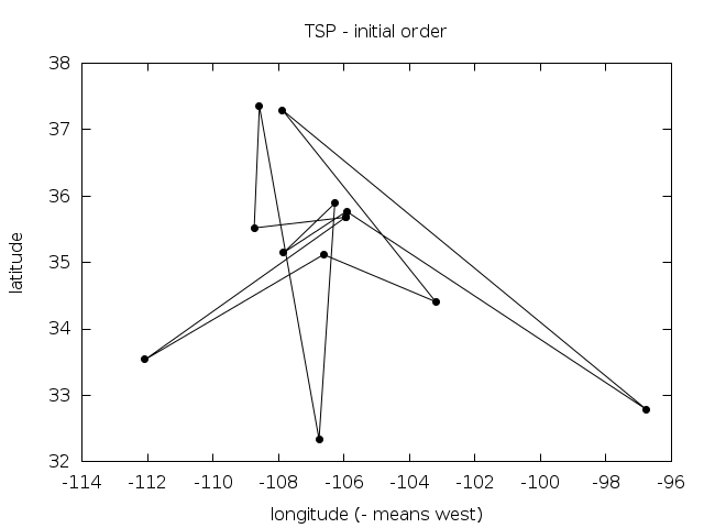
그림 14 12개의 남서부 도시를 방문하는 비행기 외판원 문제의 초기 방문 경로.
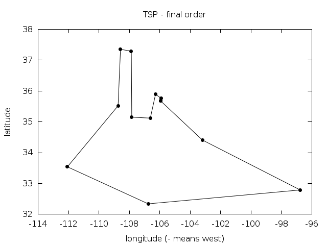
그림 15 12개의 남서부 도시를 방문하는 비행기 외판원 문제의 최종(최적화 된) 방문 경로.
다음은 비용 함수(에너지) vs 시행 횟수 그래프입니다. (각 지점은 새로운 온도가 설정되는 계산 지점을 의미합니다.)
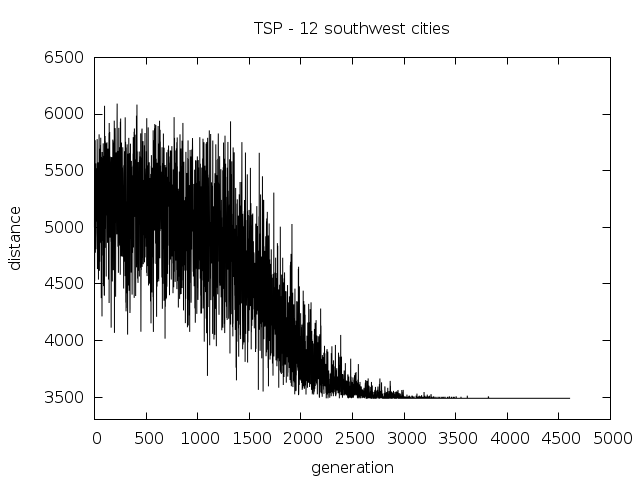
그림 16 12개의 남서부 도시를 방문하는 비행기 외판원 문제의 담금질 방법 실행 결과.
참고 문헌과 추가 자료
더 자세한 사항은 다음의 책을 참고할 수 있습니다.
Modern Heuristic Techniques for Combinatorial Problems, Colin R. Reeves (ed.), McGraw-Hill, 1995 (ISBN 0-07-709239-2).
- 1
해발고도를 재는 기준이 되는 지구의 구형 높이 입니다(*).